
Let’s summarize and compare what we’ve already learned. Then we’ll show how the various equations work together or eventually become the same thing. With a high savings rate, all roads lead to a secure financial future.
Glossary of Equations
Your savings rate, p, is the proportion of your take-home pay you save each year (excluding taxes). Your savings ratio, R, is the ratio of your savings over your spending. They relate as follows.
R=\frac{p}{1-p},~~0 < p < 1~~~~\textrm{and}~~~~p=\frac{R}{R+1}For example, calculate R as current annual savings divided by as-of-yet unsupported retirement spending. Then compute p=\frac{R}{R+1} based on that. Leave your portfolio out of this step, as it’ll be included in a few paragraphs (i.e. progress).
Starting from scratch
To reach financial independence and retire early requires 25 times annual expenses in savings, properly invested. Given the values of p and R defined above, one might expect this to happen in approximately N years.
N=-25\cdot\ln(p)After some progress
After some amount of progress, say with q proportion of the required savings in hand, the estimates above can be updated to p', R', and a new N.
\begin{darray}{rcl}p' &=& q + (1-q)\cdot p = \frac{R+q}{R+1}\\\\R' &=& \frac{R+q}{1-q} = \frac{p'}{1-p'}\\\\N &=& -25\cdot\ln(p') = -25\cdot\ln(q + (1-q)\cdot p)\end{darray}As progress builds (q\to1), the effective savings rate p' inches steadily upward even faster (p'\to1 as q\to1). Once p or p' exceeds 0.90ish, there’s a simpler way to update N.
N=\frac{25\cdot(1-p')}{p'} = \frac{25}{R'}~~\textrm{for large $p'$}All Roads Lead to (1,0)
Let’s compare the plots of our original without-interest equation (in Introducing The Savings Ratio) to our with-interest version (in Best Retirement Calculator).
\frac{25}{R}~~~~\textrm{vs}~~~~-25\cdot\ln(p)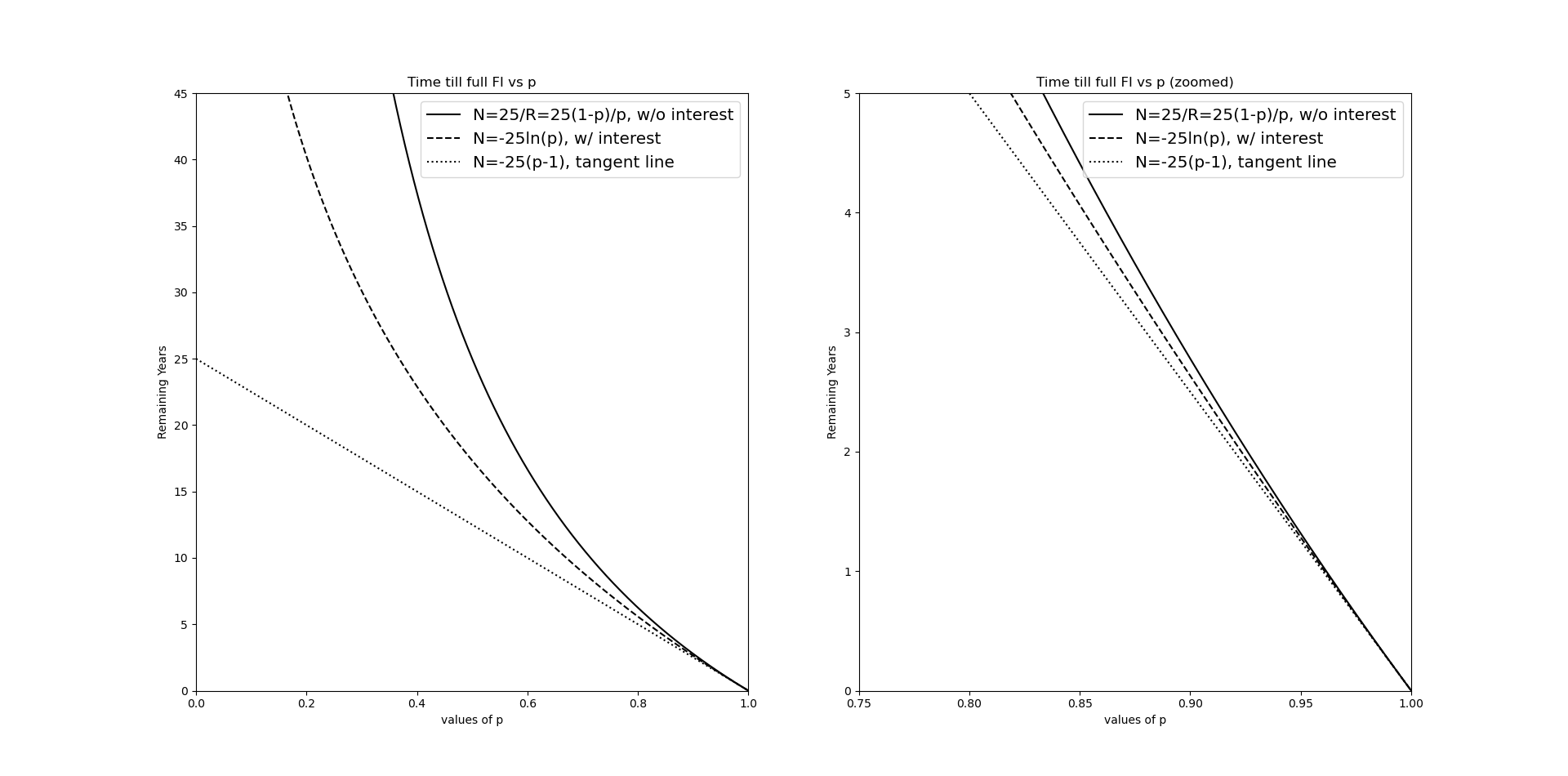
Python to generate the above pictures
import matplotlib.pyplot as plt
from math import log as ln
step = .0001
x = [x * step for x in range(1,int(1/step))]
def fi(x): return [-25*ln(p) for p in x]
def save(x): return [25*(1-p)/p for p in x]
def tangent(x): return [-25*(p-1) for p in x]
fig, (ax1,ax2) = plt.subplots(1,2)
ax1.plot(x, save(x), ‘k’, label=’N=25/R=25(1-p)/p, w/o interest’)
ax1.plot(x, fi(x), ‘k–‘, label=’N=-25ln(p), w/ interest’)
ax1.plot(x, tangent(x), ‘k:’, label=’N=-25(p-1), tangent line’)
ax2.plot(x, save(x), ‘k’, label=’N=25/R=25(1-p)/p, w/o interest’)
ax2.plot(x, fi(x), ‘k–‘, label=’N=-25ln(p), w/ interest’)
ax2.plot(x, tangent(x), ‘k:’, label=’N=-25(p-1), tangent line’)
legend = ax1.legend(loc=’upper right’, fontsize=’x-large’)
legend = ax2.legend(loc=’upper right’, fontsize=’x-large’)
ax1.set_title(‘Time till full FI vs p’)
ax1.set(xlabel=’values of p’, ylabel=’Remaining Years’)
ax1.axis((0,1,0,45))
ax2.set_title(‘Time till full FI vs p (zoomed)’)
ax2.set(xlabel=’values of p’, ylabel=’Remaining Years’)
ax2.axis((.75,1,0,5))
plt.show()
Bear in mind, these equations work just as well for the original p and R as they do for the updated versions p' and R'. In either case, they’re telling us how much longer, starting now.
Included is the tangent line, drawn in dots, to which both equations eventually converge. Observe both time estimates follow the same basic shape. The solid line does not benefit from interest compounding over the years; your savings is the only thing working in this case. So it’s natural that the with-interest dashed version gives smaller time estimates. However, as p or p' get large, say above 0.9, all three curves are nearly indistinguishable. This is because there isn’t enough time left for compounding to do its work. With so little time remaining, the without-interest version works just as well as the with-interest version. Nothing exciting is happening (hopefully) during the landing process when your jet is only 25 feet above the runway.
Further discussion
Every time you update your estimate, you hope to see a higher p' which yields a smaller length of time remaining. Given market gyrations, however, q will bounce around somewhat causing p' to do the same.
I love the N=25/R equation for its utter simplicity. The proof is enlightening to the benefits of a high savings rate. While it is an unreasonable simplification for the long term, it describes the majority of the dynamic once your effective savings rate enters the final decile (i.e. the final approach). However, after seeing the tangent line in the zoomed plot, I might start using the tangent, N=-25\cdot(p-1), for “on the run” discussions.
Given market gyrations will move things about, we’ll make this a probabilistic statement. For every final 0.01 remaining to get p'\to1, we expect the journey to take an additional quarter year. Now, in reality, when you’re that close to the finish, the market will pop you above your goal on a fairly regular basis.
Summary
We’ve seen so many equations over the last few posts that this should help pull it all together and show when to apply what.